Quotes
Every property can be classified as emergent for a sufficiently stupid observer.
La mère du maire est allée à la mer.
1, 1, 2, 5, 14, 42, 132, 429, 1430, 4862, … BIS
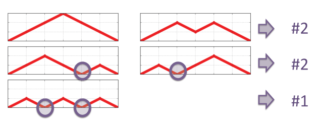
The Bernoulli excursions for 6 steps, enumerated by the Catalan sequence for n=3.
We have 5 different excursions, leaving the x-axis at the first move and coming back
after 6 moves. Some of them come back to the x-axis during the trip.
The colums of the Catalan triangle classify the excursions according to the number of times they come back during the trip: 2 times (#1), 1 times (#2) and zero times (#2). The line to be used in the case of n=3 is the line n=2 of the triangle shown in the previous post.
1, 1, 2, 5, 14, 42, 132, 429, 1430, 4862, …
Catalan numbers are an interesting sequence of integers, among many applications they have in counting problems they enumerate the celebrated Bernoulli excursions.
The n-th Catalan number can be obtained using the Catalan triangle:
n\k_____0_______1_______2_______3_______4_______5_______6_______7
0_______1
1_______1_______1
2_______1_______2_______2
3_______1_______3_______5_______5
4_______1_______4_______9_______14______14
5_______1_______5_______14______28______42______42
6_______1_______6_______20______48______90______132_____132
7_______1_______7_______27______75______165_____297_____429_____429
Each element in the triangle is obtained taking what he has at his
left plus what he has on the top.
Each column of the triangle has a nice counting property, it enumerates the subset
of Bernoulli excursions touching the x-axis a fixed number of times.
The leftmost column counts for the single Bernoulli excursion touching the maximum number of times the x-axis whilst the rightmost column enumerates the excursions with minimum number of times. The inner columns enumerate all the intermediate cases …
next post for a picture to show this in practice 🙂
GOING SMOOTHER
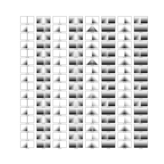
With an additive rule adding one or zero according to
an ordering between the cell and its two near neighbors we get 1024 different
CA. The plots seems smoother and the complexity lower than in the cases shown before.
Rule 364 shows some familiar triangular structure but fading away …
As for the previous post … to generate the plots above, I used the following rattlesnake script:
# Script to generate simple Cellular Automata
# PL 26.VI.2015

import numpy as np
import matplotlib.pyplot as plt

# Aux Functions
########################################

def rule_creator_1024(rule):

    a = map(int,bin(rule)[2:].zfill(10)) # rule creator

    return a


def CA(rule,cells3):

    a = cells3[0];
    b = cells3[1];
    c = cells3[2];

    if ( a > b) & (a > c ) & ( b > c)  : nn = 0
    if ( a > b) & (a > c ) & ( b < c)  : nn = 1

    if ( b > a) & (b > c ) & ( a > c)  : nn = 2
    if ( b > a) & (b > c ) & ( a < c)  : nn = 3

    if ( c > a) & (c > b ) & ( a > b)  : nn = 4
    if ( c > a) & (c > b ) & ( a < b)  : nn = 5

    if ( a == b)                       : nn = 6
    if ( b == c)                       : nn = 7
    if ( a == c)                       : nn = 8
    if ( a == b) & (a == c)            : nn = 9
    return rule[nn]

# Main program
########################################

N=30 # Number of Cellular Automata Steps

# memory matrix init

dat=np.zeros([N,N*4+1],np.int)

dat[0,2*N]=1;

cells3=[0,0,0];

plt.figure(figsize=(20, 20))

# do the job

counter = 0

for rule in range(1024):

    print "Rule Number -->", rule

    plt.subplot(16,8,(rule)%128+1)

    res=rule_creator_1024(rule)

    for stp in np.arange(1,N):
        for i in np.arange(1,4*N):

            cells3[0]  = dat[stp-1,i-1];
            cells3[1]  = dat[stp-1,i];
            cells3[2]  = dat[stp-1,i+1];

            dat[stp,i] = dat[stp-1,i] + CA(res,cells3);                 # apply the Cellular Automata with rule --> res

#   completed one realization ...

    dat_to_plot=dat[:,N+1:3*N].copy()                    # plot only the central window

    plt.gca().xaxis.set_major_locator(plt.NullLocator()) # remove ticks and labels
    plt.gca().yaxis.set_major_locator(plt.NullLocator())

    plt.pcolor(dat_to_plot[::-1], cmap='Greys')

    rulenm='rule ' + str(rule); plt.xlabel(rulenm,fontsize='xx-small')

    if (counter+1)%128 == 0: #plot first page
        file_out = 'plot_' + str(counter-127).zfill(3) + '_' + str(counter).zfill(3) + '.png'
        plt.savefig(file_out, format='png',dpi=900)
        plt.clf()
        plt.figure(figsize=(20, 20))


    counter = counter +1;

print 'EOB'
Another brick in the wall
The four types of CA classes namely the trivial (1), the periodic (2), the chaotic (3), and the mix between the period and chaotic (4) should constitute quite a general classification.
I did some tests adding a wall on the left side of the grid … now there are 256 * 8 stamps available, according to the 8 different rules applied at the wall … (I will not post all of them)
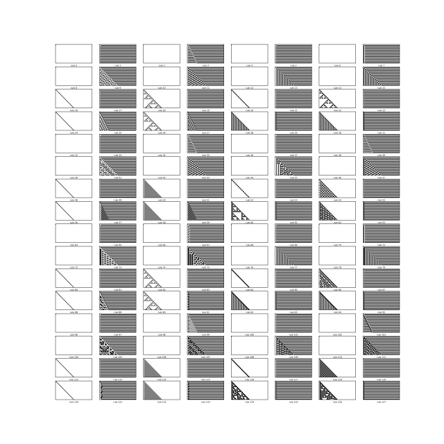
It should be essentially the same level of complexity as in the previous post at least according to the “mantra” by Stephen W.
I will print this stuff and give a look.
As for the previous post … to generate the plots above, I used the following python script:
# Script to generate simple Cellular Automata
# with a wall in the left side of each stamp
# PL 13.VI.2015

import numpy as np
import matplotlib.pyplot as plt

# Aux Functions
########################################

def rule_creator_8(rule):

    a = map(int,bin(rule)[2:].zfill(4)) # rule creator

    return a

def rule_creator_256(rule):

    a = map(int,bin(rule)[2:].zfill(8)) # rule creator

    return a


def CA(rule,cells):

    if len(cells) == 2:
        a = (-cells[0]+1) * 2 + (-cells[1]+1);

    if len(cells) == 3:
        a = (-cells[0]+1) * 4 + (-cells[1]+1) *2 + (-cells[2]+1);

    return rule[a]

# Main program
########################################

N=30 # Number of Cellular Automata Steps

# memory matrix init

dat=np.zeros([N,N*3+1],np.int)

dat[0,0]=1;

cells3=[0,0,0];
cells2=[0,0];

plt.figure(figsize=(20, 20))

# do the job

counter = 0;

for rule2 in range(8):

    res2=rule_creator_8(rule2)

    for rule3 in range(256):

        print "Rule Number -->", rule2, " --- ", rule3

        plt.subplot(16,8,(rule3)%128+1)

        res3=rule_creator_256(rule3)

        for stp in np.arange(1,N):

            cells2[0]  = dat[stp-1,0];
            cells2[1]  = dat[stp-1,1];

            dat[stp,0] = CA(res2,cells2);                 # apply the Cellular Automata with rule --> res

            for i in np.arange(1,3*N):

                cells3[0]  = dat[stp-1,i-1];
                cells3[1]  = dat[stp-1,i];
                cells3[2]  = dat[stp-1,i+1];

                dat[stp,i] = CA(res3,cells3);                 # apply the Cellular Automata with rule --> res

#   completed one realization ...

        dat_to_plot=dat[:,0:2*N].copy()                    # plot only the central window

        plt.gca().xaxis.set_major_locator(plt.NullLocator()) # remove ticks and labels
        plt.gca().yaxis.set_major_locator(plt.NullLocator())

        plt.pcolor(dat_to_plot[::-1], cmap='Greys')

        rulenm='rule ' + str(rule3); plt.xlabel(rulenm,fontsize='xx-small')

        if (counter+1)%128 == 0: #plot first page
           file_out = 'plot_' + str(counter-127).zfill(3) + '_' + str(counter).zfill(3) + '.png'
           plt.savefig(file_out, format='png',dpi=900)
           plt.clf()
           plt.figure(figsize=(20, 20))


        counter = counter +1;

print 'EOB'
SIMPLE RULES – ANKS plots
